Mastering Query Rewriting for Faster PostgreSQL Performance

When you first spin up your app, the emphasis is on getting started and getting data to your clients. But when you don’t have throughput, you are also not going to have enough concurrency to unveil bad queries.

But then you have success. And success means data. More users, more interactions, more everything. Suddenly, queries that performed fine are struggling under the load, hurting performance and scalability. This is all going to mean a far worse user experience when much higher costs because of inefficient resource use.

This is where mastering query rewriting techniques comes into play. By analyzing and refactoring your SQL queries, you can significantly improve the performance of your PostgreSQL database. Query optimization and rewriting can also reduce query execution times, minimize resource consumption, and efficiently handle larger datasets. 

Let’s go through a few options here, looking at the performance gains they can provide and other options available to database engineers.

Faster PostgreSQL Performance Through Indexing

Let’s start with our query. Let’s say we have a products table and a sales table, and we want to calculate the total sales amount for each product category for last year. 

SELECT p.category_id, SUM(s.quantity * p.price) AS total_sales
FROM sales s
JOIN products p ON s.product_id = p.product_id
WHERE s.sale_date BETWEEN '2023-01-01' AND '2023-12-31'
GROUP BY p.category_id

This isn’t a crazy complicated query. But it is inefficient. As products grows into thousands of rows and sales into millions, the time for this query to run gets into seconds:

Time: 1300.403 ms (00:01.300)

Again, it's not bad, but it will only get worse. To get a better understanding of what is happening under the hood, we can run this query with EXPLAIN ANALYZE to output the query plan:

PLAN                                                                         
--------------------------------------------------------------------------------------------------------------------------------------------------------
 Finalize GroupAggregate  (cost=158598.39..158624.47 rows=100 width=36) (actual time=1346.917..1348.210 rows=100 loops=1)
   Group Key: p.category_id
   ->  Gather Merge  (cost=158598.39..158621.72 rows=200 width=36) (actual time=1346.909..1348.108 rows=300 loops=1)
         Workers Planned: 2
         Workers Launched: 2
         ->  Sort  (cost=157598.36..157598.61 rows=100 width=36) (actual time=1337.800..1337.803 rows=100 loops=3)
               Sort Key: p.category_id
               Sort Method: quicksort  Memory: 34kB
               Worker 0:  Sort Method: quicksort  Memory: 34kB
               Worker 1:  Sort Method: quicksort  Memory: 34kB
               ->  Partial HashAggregate  (cost=157593.79..157595.04 rows=100 width=36) (actual time=1337.710..1337.725 rows=100 loops=3)
                     Group Key: p.category_id
                     Batches: 1  Memory Usage: 80kB
                     Worker 0:  Batches: 1  Memory Usage: 80kB
                     Worker 1:  Batches: 1  Memory Usage: 80kB
                     ->  Hash Join  (cost=280.00..126235.13 rows=3135866 width=14) (actual time=4.633..874.357 rows=2510665 loops=3)
                           Hash Cond: (s.product_id = p.product_id)
                           ->  Parallel Seq Scan on sales s  (cost=0.00..117720.00 rows=3135866 width=8) (actual time=0.194..583.607 rows=2510665 loops=3)
                                 Filter: ((sale_date >= '2023-01-01'::date) AND (sale_date <= '2023-12-31'::date))
                                 Rows Removed by Filter: 856002
                           ->  Hash  (cost=155.00..155.00 rows=10000 width=14) (actual time=4.339..4.339 rows=10000 loops=3)
                                 Buckets: 16384  Batches: 1  Memory Usage: 597kB
                                 ->  Seq Scan on products p  (cost=0.00..155.00 rows=10000 width=14) (actual time=0.129..1.971 rows=10000 loops=3)
 Planning Time: 0.767 ms
 Execution Time: 1348.468 ms
(25 rows)

The first option here isn't so much a rewrite as a simple optimization: indexing. Indexing allows PostgreSQL to quickly locate and retrieve relevant data without scanning the entire table. By creating indexes on frequently used columns, such as product_id in both the sales and products tables, query performance can be improved.

CREATE INDEX idx_sales_product_id ON sales (product_id);
CREATE INDEX idx_products_product_id ON products (product_id);

By adding these indexes, PostgreSQL can efficiently locate the relevant rows based on the specified conditions, reducing the need for full table scans. This can lead to a significant reduction in query execution time, especially for large datasets. The time with these simple indexes is:

Time: 1211.155 ms (00:01.211)

Hmm, not quite the performance gain expected. Why?

The performance gain is not as significant as expected because while the indexes on the product_id columns help with the join operation, the query still needs to perform a scan on the sales table to filter the rows based on the sale_date condition. The WHERE clause s.sale_date BETWEEN '2023-01-01' AND '2023-12-31' requires scanning all the rows in the sales table to determine which ones fall within the specified date range. We can see this in the query plan (so we could have skipped the above indexes, but we’re just playing here!)

To further optimize the query, we can create a composite index on the product_id and sale_date column in the sales table:

CREATE INDEX idx_sales_product_id_sale_date ON sales(product_id, sale_date);

A composite index can be particularly effective for queries like this that join on product_id and filter on sale_date, as it can help the database efficiently locate the relevant rows based on both criteria. With the composite index, we do get a better performance gain:

Time: 844.296 ms

What are the problems with indexes? While indexes can significantly improve query performance, they come with some trade-offs. First, they consume additional storage space on disk, as they store a copy of the indexed columns along with a pointer to the original table. This can increase the overall database size, especially if multiple indexes are created on large tables.

Second, when a row is inserted, updated, or deleted, the corresponding indexes must also be updated to maintain their integrity. This can slow down write operations, particularly in write-intensive scenarios.

Lastly, indexes require careful consideration and planning. Creating too many indexes or indexing the wrong columns can negatively impact performance. Analyzing the query patterns, data distribution, and performance requirements to determine the most beneficial indexes for your specific use case is important. Over-indexing can lead to increased maintenance overhead and potentially degrade performance instead of improving it.

Faster PostgreSQL Performance Through CTEs

So, indexes didn’t work. What’s next? Query rewriting through Common Table Expressions, or CTEs, can help PostgreSQL performance by breaking down complex queries into smaller, more manageable parts. CTEs allow you to define named temporary result sets that can be referenced multiple times within the main query, improving query readability, maintainability, and, in some cases, performance.

Using CTEs, you can precompute intermediate results, filter or aggregate data before joining with other tables, and avoid redundant calculations. This can lead to more efficient query execution plans and faster query performance, especially for queries involving multiple subqueries or complex joins.

Let's see how we can rewrite our original query using CTEs to potentially improve its performance:

WITH filtered_sales AS (
   SELECT s.product_id, s.quantity, s.price
   FROM sales s
   JOIN products p ON s.product_id = p.product_id
   WHERE s.sale_date BETWEEN '2023-01-01' AND '2023-12-31'
)
SELECT category_id, SUM(quantity * price) AS total_sales
FROM filtered_sales
JOIN products p ON filtered_sales.product_id = p.product_id
GROUP BY category_id;

This gets us:

Time: 1787.937 ms

What? That doesn’t seem faster. That looks slower. What’s up? 

The CTE version introduces an additional step in the query execution plan–the CTE Scan on filtered_sales. This step materializes the intermediate result set generated by the CTE, which includes the join between the sales and products tables and the filtering based on the sale_date condition.

While CTEs can be beneficial in specific scenarios, in this case, the materialization of the intermediate result set adds overhead to the query execution. In this particular query, using a CTE does not provide any performance benefits and instead introduces additional overhead. This is an excellent example of the PostgreSQL query optimizer already working to improve your queries and run them most efficiently. Adding steps that seem optimal can screw with internal optimizations, leading to slower performance.

Faster PostgreSQL Performance Through Materialized Views

The next option is materialized views. Materialized views are precomputed result sets stored physically on disk and can be refreshed periodically. They act as a snapshot of the data at a particular point in time and can be queried like regular tables.

By creating a materialized view that contains the aggregated sales data grouped by product category, we can avoid the overhead of performing the join and aggregation operations every time the query is executed. The materialized view can be refreshed at a scheduled interval or manually to keep the data current.

Here's how we can create a materialized view for our query:

CREATE MATERIALIZED VIEW category_sales_summary AS
SELECT p.category_id, SUM(s.quantity * p.price) AS total_sales
FROM sales s
JOIN products p ON s.product_id = p.product_id
WHERE s.sale_date BETWEEN '2023-01-01' AND '2023-12-31'
GROUP BY p.category_id;

Once the materialized view is created, we can query it directly:

SELECT * FROM category_sales_summary;

This approach can significantly improve query performance by eliminating the need for real-time joins and aggregations. See:

Time: 3.700 ms

Boom. Success. Materialize all the views.

But there are trade-offs. Materialized views consume additional storage space since they store a separate copy of the precomputed result set. This can increase disk usage, especially if the materialized views are large or numerous.

More importantly, materialized views must be refreshed to keep the data current. Depending on the frequency of data changes and the refresh strategy, there may be a lag between the actual data and the data in the materialized view. If the materialized view is not refreshed frequently enough, it can serve stale data to users.

Lastly, maintaining materialized views adds complexity. You need to consider the refresh schedule, the impact of data modifications on the materialized views, and the potential need to rebuild them if the underlying data structure changes significantly.

Faster PostgreSQL Performance Through Readyset

All of the above work in some variation, but they all have a simple problem: they are time-consuming. Here, we’re talking about optimizing a single, simple query, but any application will have dozens of queries with varying complexities. 

Running through this list of query rewriting techniques for each query and looking for a few milliseconds of improvement isn’t a good use of your team’s time. They should be building product, not working as DBAs.

The answer? Readyset. With Readyset, you can get faster PostgreSQL performance without spending time mastering query rewriting. To set this up to work with Readyset, we first need to add Readyset as a replication instance of our database. You can either do this using Readyset Cloud or locally using:

docker run -d -p 5433:5433 -p 6034:6034         \
--name readyset                                 \
-e UPSTREAM_DB_URL=<database connection string> \
-e REPLICATION_TABLES=<specific tables or omit> \
-e LISTEN_ADDRESS=0.0.0.0:5433                  \
readysettech/readyset:latest

This will start creating a snapshot of your tables. When this is completed, you can connect to Readyset just as you would connect to your primary database, as Readyset is wire-compatible with Postgres:

psql 'postgresql://<username>:<password>@<readyset_host>:5433/<database> 

We can then run the same query above, which will initially be proxied through Readyset. When we’ve done that, we can use SHOW PROXIED QUERIES; to see if Readyset supports the query (see supported queries to learn more about what you can currently use with Readyset):

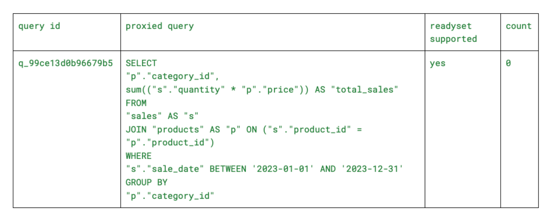
If readyset supported is yes, then we can use CREATE CACHE FROM to create our cache:

CREATE CACHE FROM SELECT p.category_id, SUM(s.quantity * p.price) AS total_sales
FROM sales s
JOIN products p ON s.product_id = p.product_id
WHERE s.sale_date BETWEEN '2023-01-01' AND '2023-12-31'
GROUP BY p.category_id;

Now, when we run that query, we get a considerable performance gain:

Time: 14.818 ms

By caching our query with Readyset, we’ve seen a 100X performance improvement (and this is on an M1 Mac, with the performance tradeoff from the Docker emulation). We are on the same order of magnitude as materialized views (which makes sense as Readyset creates a materialized view) but without the management overhead. Readyset will keep our cache up to date with all data manipulations–INSERTs, UPDATEs, and DELETEs–that happen in the primary database. No extra work on our side–the data will always be fresh, and your engineers won’t have to do anything.

Remove Rewriting From Your Team’s Backlog

Query rewriting is one of those tasks that will always be in the backlog. Either someone on your team takes it on and invests time and resources to make the slight improvements you see above, or it continues to sit there, deteriorating your performance and user experience.

With Readyset, you can 100X your query performance in minutes with no changes to your SQL code or application layer. With wire compatibility, all your engineers need to do is change their connection string, and they can see immediate performance gains.

If you’re done with query rewriting and this sounds good, sign up for Readyset Cloud or get started locally with Docker.